Distribucion espacial de poblacion en riesgo
Analisis de los datos del INEI sobre la distribucion de las personas mayores de 60 años.
Datos Handbook Covid-19 Perú
Informacion Adicional Gobierno del Peru
Situacion Nivel Mundial Coronavirus COVID-19 Global Cases by the Center for Systems Science and Engineering (CSSE)
Datos
library(tidyverse)
library(sf)

area.sf1 <- st_read("./_dat/per_admbnda_adm3_2018/per_admbnda_adm3_2018.shp") %>%
  mutate(NOMBDIST = str_replace_all(NOMBDIST, "Ñ", "N"),
         NOMBPROV = str_replace_all(NOMBPROV, "Ñ", "N"),
         NOMBDIST = ifelse(NOMBDIST=="MAZAMARI - PANGOA", "MAZAMARI",NOMBDIST),
         NOMBDIST = ifelse(NOMBDIST=="HUAYA", "HUALLA",NOMBDIST),
         NOMBDIST = ifelse(NOMBPROV=="HUAROCHIRI" & NOMBDIST=="LARAOS", "SAN PEDRO DE LARAOS",NOMBDIST)
) ## Reading layer `per_admbnda_adm3_2018' from data source `/Users/gcarrasco/Desktop/aa/content/post/02_spat_elderly/_dat/per_admbnda_adm3_2018/per_admbnda_adm3_2018.shp' using driver `ESRI Shapefile'
## Simple feature collection with 1873 features and 16 fields
## geometry type: MULTIPOLYGON
## dimension: XY
## bbox: xmin: -81.32823 ymin: -18.35093 xmax: -68.65228 ymax: -0.03860597
## geographic CRS: WGS 84dat <- read.csv("./_dat/spat_covid_v2.csv") %>%
mutate(NOMBDEP = toupper(dep),
NOMBPROV = toupper(prov),
NOMBDIST = toupper(dist))
dat.sf <- area.sf1 %>%
inner_join(dat %>% group_by(NOMBDEP, NOMBPROV, NOMBDIST) %>%
summarise(N = sum(N)),
by = c("NOMBDEP", "NOMBPROV", "NOMBDIST"))Figuras
library(colorspace)
library(cowplot)
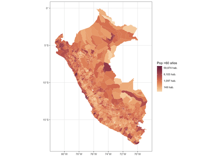
dat.sf %>%
ggplot() +
geom_sf(aes(fill=N), size = 0.05, col = NA) +
scale_fill_continuous_sequential(palette = "BurgYl", name = "Pop >60 años", trans = "log",
labels = scales::comma_format(suffix = " hab.")) +
theme_bw()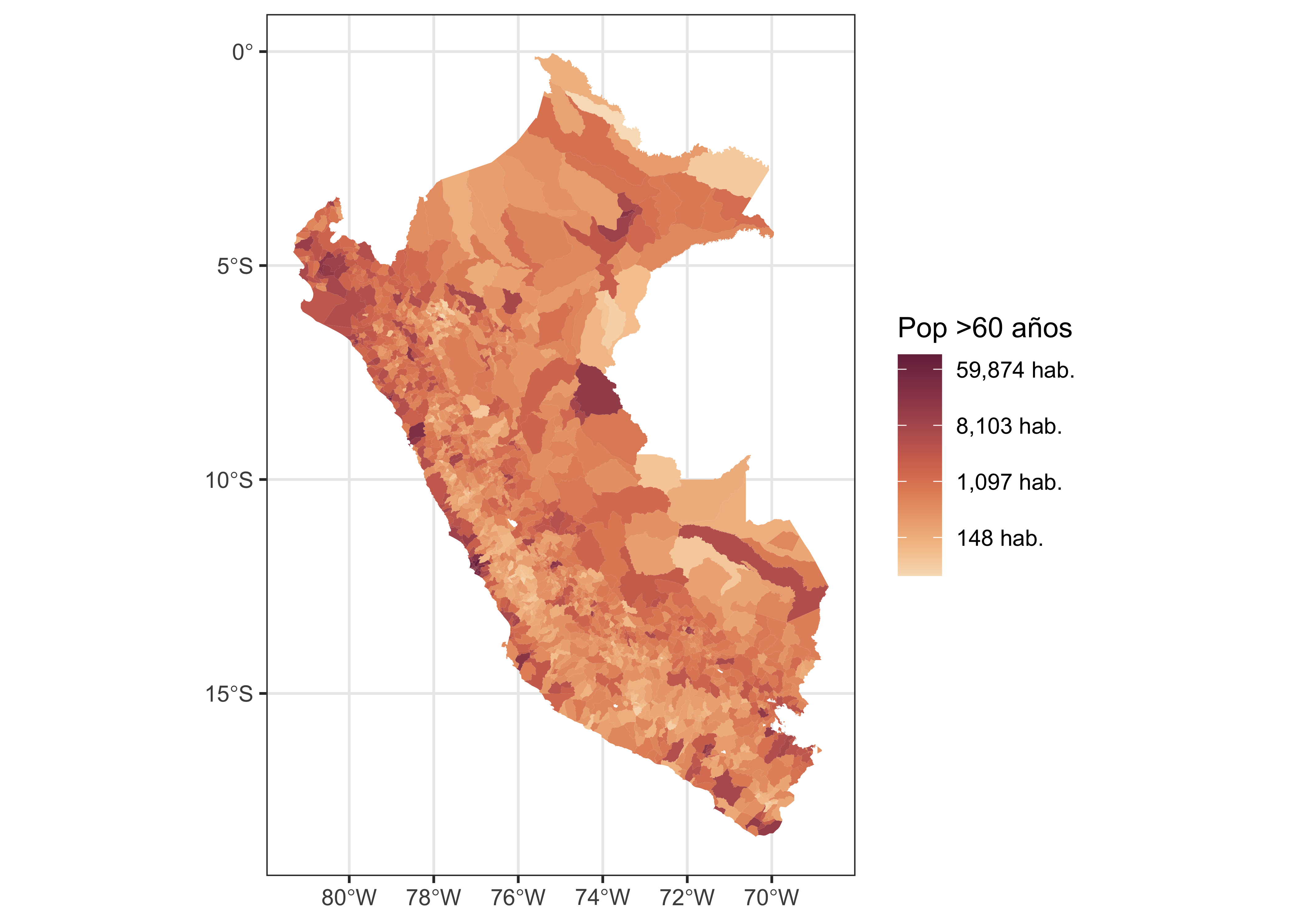
f2 <- purrr::map(unique(dat.sf$NOMBDEP),
           function(x) {
             ggplot() +
               geom_sf(data = dat.sf %>% filter(NOMBDEP == x),
                       aes(fill=N), size = 0.05, col = NA) +
               scale_fill_continuous_sequential(palette = "BurgYl", name = "Hab. >60 años", trans = "log",
                                                labels = scales::comma_format(suffix = " hab."),
                                                limits=range(dat.sf$N)) +
               guides(fill = FALSE) +
               labs(title = x) +
               theme_bw(base_size = 5)
           })

cowplot::plot_grid(plotlist = f2)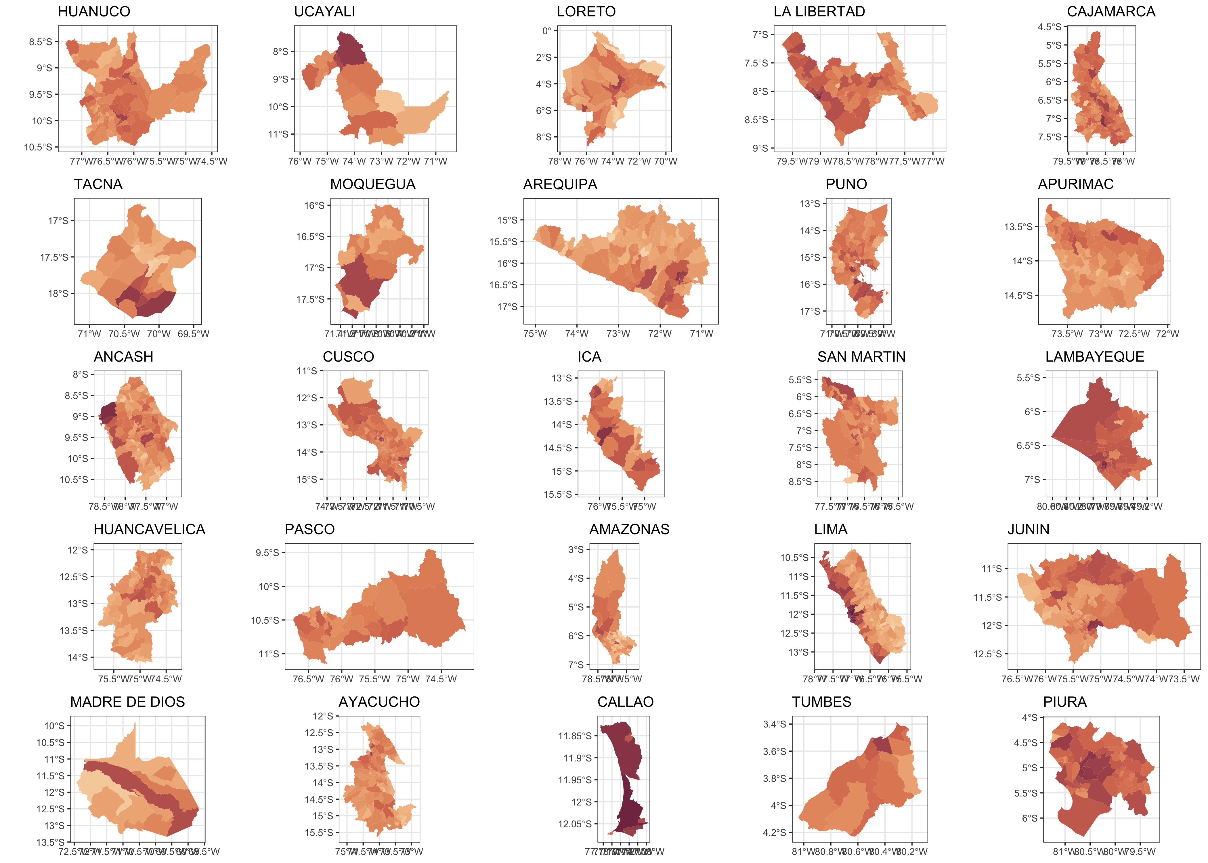
f3 <- purrr::map(c("LIMA","CALLAO"),
           function(x) {
             ggplot() +
               geom_sf(data = dat.sf %>% filter(NOMBPROV == x),
                       aes(fill=N), size = 0.05, col = NA) +
               scale_fill_continuous_sequential(palette = "BurgYl", name = "Hab. >60 años",
                                                labels = scales::comma_format(suffix = " hab.")) +
               labs(title = x) +
               theme_bw(base_size = 5)
           })

cowplot::plot_grid(plotlist = f3)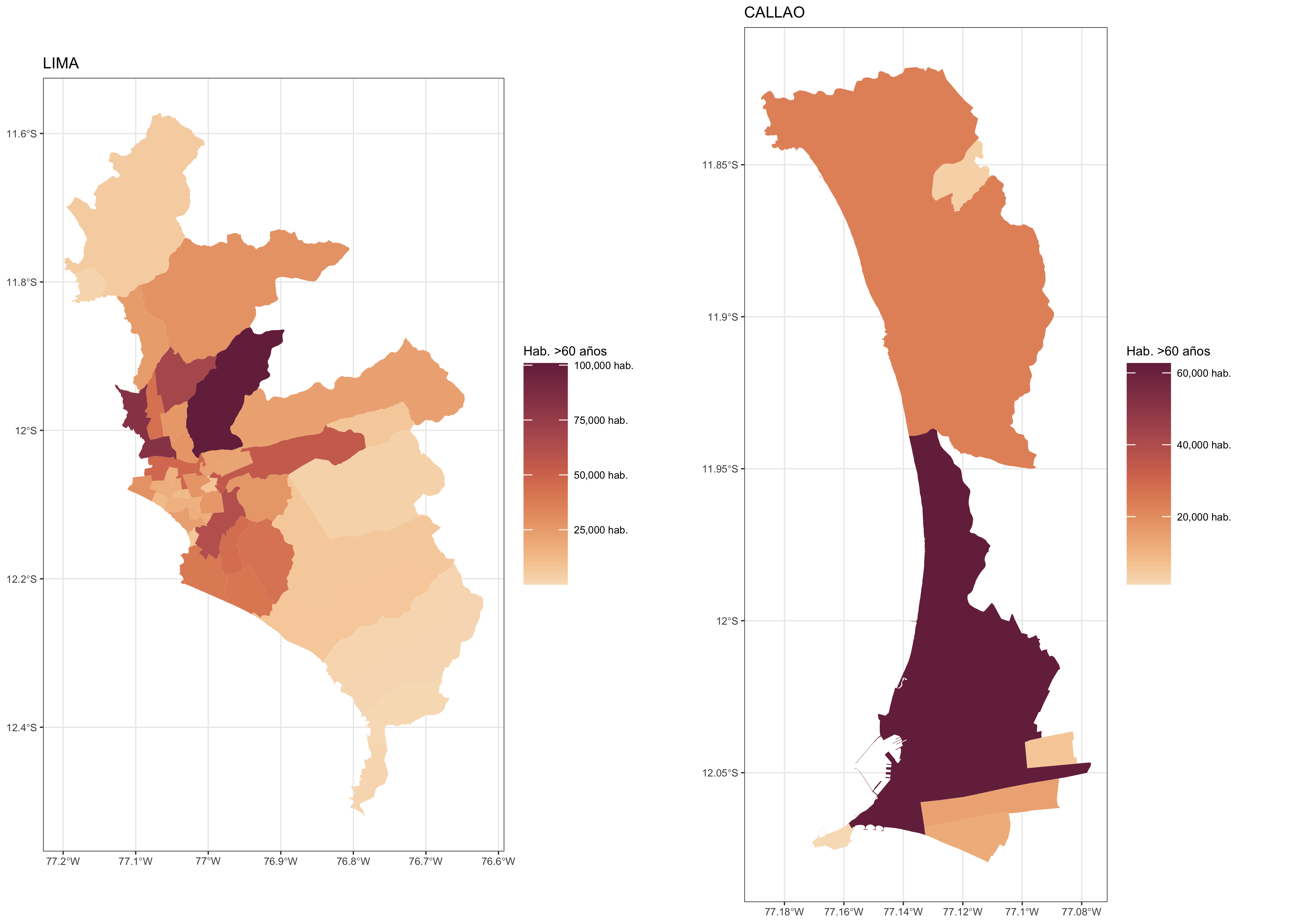
Por grupo de Edades
dat.sf2 <- area.sf1 %>%
  inner_join(dat, by = c("NOMBDEP", "NOMBPROV", "NOMBDIST"))

dat.sf2 %>%
  ggplot() +
  geom_sf(aes(fill=N), size = 0.05, col = NA) +
  scale_fill_continuous_sequential(palette = "BurgYl", name = "Pop >60 años", trans = "log",
                       labels = scales::comma_format(suffix = " hab.")) +
  theme_bw() +
  facet_grid(.~cat_age)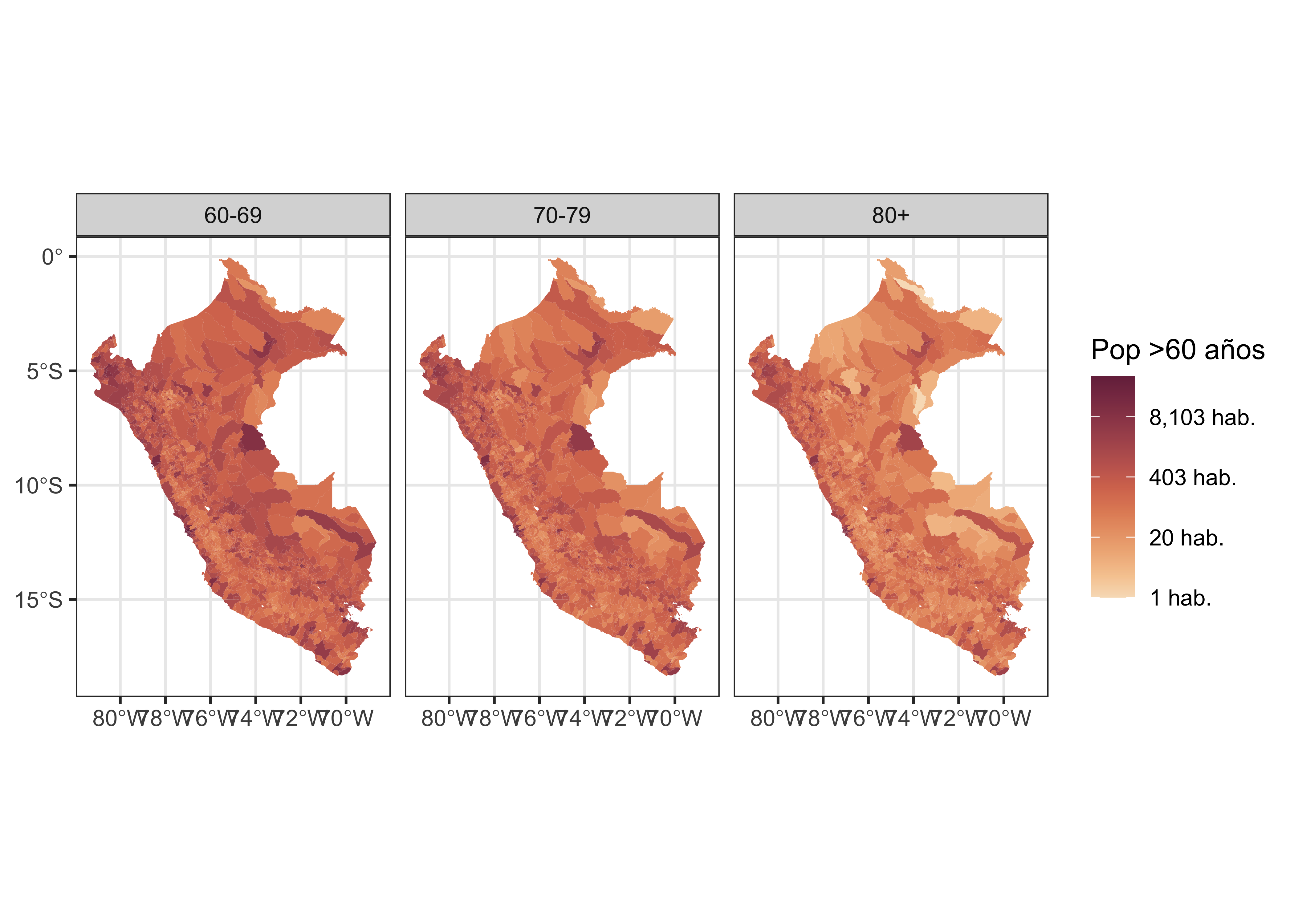
f4 <- purrr::map(c("LIMA","CALLAO"),
           function(x) {
             ggplot() +
               geom_sf(data = dat.sf2 %>% filter(NOMBPROV == x),
                       aes(fill=N), size = 0.05, col = NA) +
               scale_fill_continuous_sequential(palette = "BurgYl", name = "Hab. >60 años",
                                                labels = scales::comma_format(suffix = " hab.")) +
               labs(title = x) +
               theme_bw(base_size = 5) +
               facet_grid(.~cat_age)
           })

cowplot::plot_grid(plotlist = f4, nrow = 2)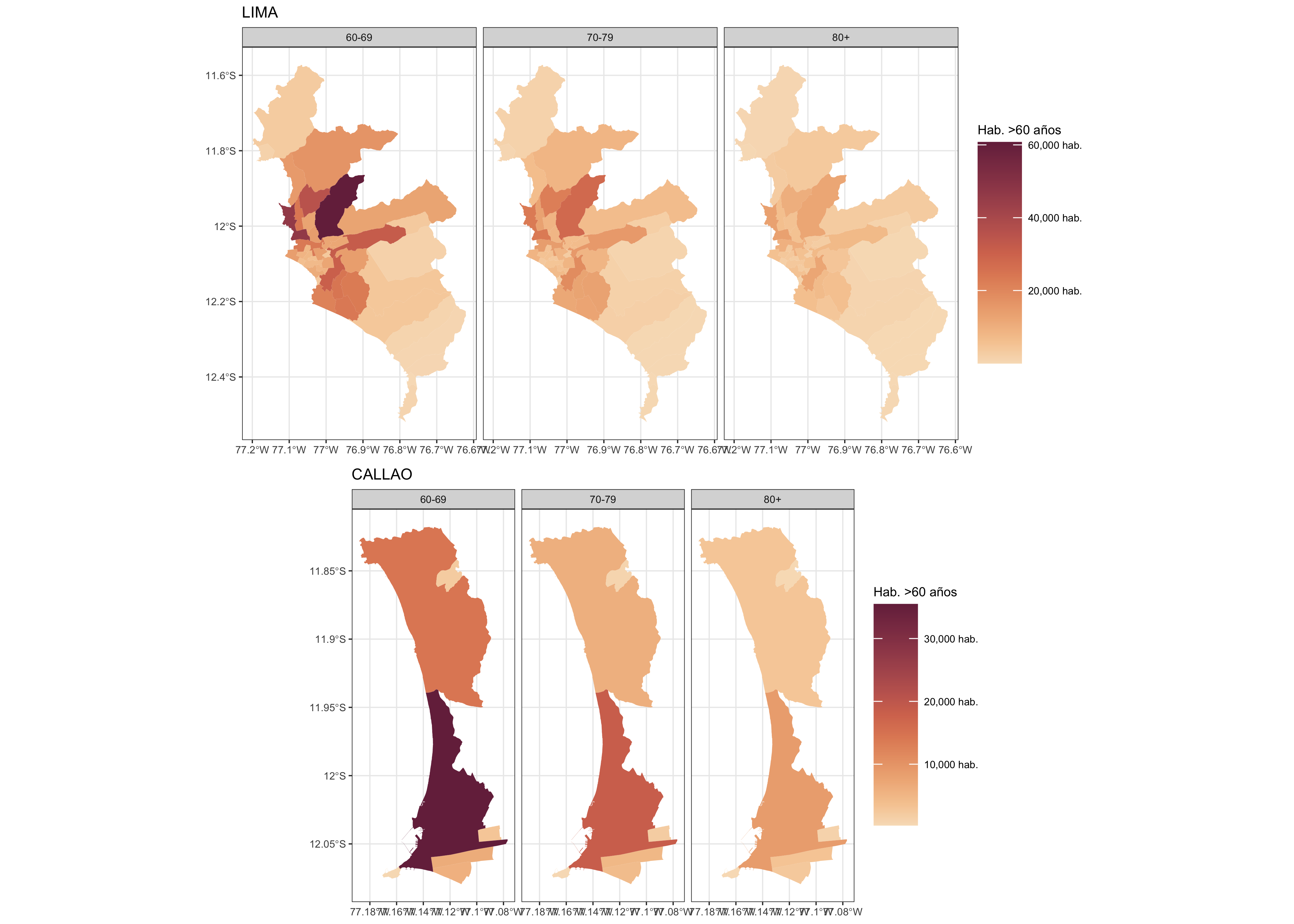
Gabriel Carrasco-Escobar
Assistant Professor
My research interests include infectious diseases epidemiology, causal inference, global health, Climate Change, Data Science, Urban Health, and Geospatial modeling & viz.